Water Ripple Simulation

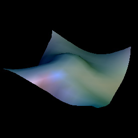
Here is a simple water ripple simulation showing single slit wave diffraction. The following Mathematica code solves the wave equation with damping using the finite difference method. You can read more about this algorithm on Hugo Elias’ website. (Note: technically this simulation should use Neumann boundary conditions but I decided it was simplier to demonstrate using Dirichlet boundary conditions).

(* runtime: 18 seconds, c is the wave speed and b is a damping factor *) n = 64; c = 1; b = 5; dx = 1.0/(n - 1); Courant = Sqrt[2.0]/2;dt = Courant dx/c; z1 = z2 = Table[0.0, {n}, {n}]; Do[{z1, z2} = {z2, z1}; z1[[n/2, n/4]] = Sin[16Pi t]; Do[If[0.45 < i/n < 0.55 || ! (0.48 < j/n < 0.52), z2[[i, j]] = (2(1 - 2Courant^2)z1[[i, j]] + Courant^2(z1[[i - 1, j]] + z1[[i + 1, j]] + z1[[i, j - 1]] + z1[[i, j + 1]]))/(1 + b dt) - z2[[i, j]]], {i, 2, n - 1}, {j, 2, n - 1}]; ListPlot3D[z1, Mesh -> False, PlotRange -> {-1, 1}], {t, 0, 1, dt}];

Links

• Water Figures – beautiful high-speed camera splashes by Fotoopa
• LSSM – POV-Ray animations using this same technique, by Tim Nikias Wenclawiak
• POV-Ray Ripples – another one by Rune Johansen
• Water Ripples – Delphi program by Jan Horn
• Waves – C++ program by Maciej Matyka
• Fluid Animations – amazing animations by Ron Fedkiw, with Eran Guendelman, Andrew Selle, Frank Losasso, et al.
• Free Surface Fluid Simulations – impressive simulations using the Lattice-Boltzmann method with level sets, by Nils Thuerey, author of Blender’s fluid package
• Fluid v1.0 – C++ program for fluid surfaces by Maciej Matyka, uses Marker And Cell (MAC) method
• ball in water – nice 3D POV-Ray animation by Fidos
• Splash – analytical Mathematica plot by Dr. Jim Swift
• Smoke Animations – by Jos Stam, Henrik Jensen, Ron Fedkiw, et al.
• Fire Animations – by Duc Nguyen, Henrik Jensen, Ron Fedkiw

Raindrop Light Dispersion

When light enters near the side of a raindrop, much of the light is internally reflected. This is how rainbows are formed. You can also see this animation on Jeff Bryant’s Mathematica visualization site.

Raindrop Light Dispersion – Mathematica 4.2, 1/21/05;
C++ version: 7/26/05

(* runtime: 12 seconds *)
Spectrum = {{380, {0, 0, 0}}, {420, {1/3, 0, 1}}, {440, {0, 0, 1}}, {490, {0, 1, 1}}, {510, {0, 1,0}}, {580, {1, 1, 0}}, {645, {1, 0, 0}}, {700, {1, 0, 0}}, {780, {0, 0, 0}}};
Snell[theta_, n1_, n2_] := ArcSin[Min[1, Max[-1, Sin[theta]n1/n2]]];
FresnelR[t1_, t2_, n1_, n2_] := (((n1 Cos[t2] - n2 Cos[t1])/(n1 Cos[t2] + n2 Cos[t1]))^2 + ((n1 Cos[t1] - n2 Cos[t2])/(n1 Cos[t1] + n2 Cos[t2]))^2)/2;
Angle[{x1_, y1_}, {x2_, y2_}] := ArcTan[x2 - x1, y2 - y1];
IntersCircle[{x_, y_}, theta_, {x0_,y0_}, r_] := Module[{t1 = Tan[theta], t2, a, b, x2}, t2 = ((x -x0) t1 - (y - y0))/r; a = t1^2 + 1; b = -2t1 t2; x2 = x0 + r(-b + If[Cos[theta] > 0, 1, -1]Sqrt[b^2 - 4a (t2^2 - 1)])/(2a); {x2, y + (x2 - x)t1}];
AddLine[{x1_, y1_}, {x2_, y2_}, color_] := Do[image[[Round[m(s y1 + (1 - s) y2)], Round[m(s x1 + (1 - s)x2)]]] += color, {s, 0,1, 1/(m Sqrt[(x2 - x1)^2 + (y2 - y1)^2])}];
m = 275; image =Table[{0, 0, 0}, {m}, {m}]; x0 = y0 = 0.5; p0 = {x0, y0}; r = 0.25;
Do[n = 1.31Exp[12.4/lambda]; color = Table[Interpolation[Map[{#[[1]], #[[2, i]]} &, Spectrum], InterpolationOrder -> 1][lambda], {i, 1, 3}]; p1 = {x0 - Sqrt[r^2 - (y - y0)^2], y}; t = Angle[p0, p1]; t1 = t + Snell[Pi - t, 1,n] - Pi; While[Max[color] > 0.01, p2 = IntersCircle[p1, t1, p0, r]; AddLine[p1,p2, color]; t = Angle[p0, p2]; t2 =2t - t1 - Pi; t3 = t - Snell[t - t1, n, 1]; R1 = FresnelR[t - t1, t -t3, n, 1]; AddLine[p2, IntersCircle[p2, t3, p0, 0.49], (1 - R1) color]; p1 = p2; t1 = t2; color *= R1], {lambda, 380, 780, 25}, {y, y0 + r - 0.001, y0 + r - 0.0001, 0.0001}];
Show[Graphics[RasterArray[Map[RGBColor @@ Map[Min[1, #] &, #] &, image, {2}]], Epilog -> {{RGBColor[1, 1, 1], Circle[m p0, m r]}}, AspectRatio -> 1]]

Click here to see some POV-Ray code for a similar-looking image using photon mapping.

Apollonian Gasket

Here are four circles inverted about each other. This is kind of similar to a Wada Basin but not exactly. Notice the small Poincaré hyperbolic tilings throughout the picture. Click here to download a Mathematica notebook for this animation. Click here to download some POV-Ray code for this fractal.

(* runtime: 0.3 second *)
chains = {N[Append[Table[{{2E^(I theta), Sqrt[3]}}, {theta, Pi/6, 9Pi/6, 2Pi/3}], {{0, 2 - Sqrt[3]}}]]};
Reflect[{z2_, r2_}, {z1_, r1_}] := Module[{a = r1^2/((z2 -z1)Conjugate[z2 - z1] - r2^2)}, {z1 + a (z2 - z1), a r2}];
Do[chains = Append[chains, Table[Map[Reflect[#, chains[[1, j, 1]]] &, Flatten[Delete[chains[[i]], j], 1]], {j, 1, 4}]], {i, 1, 6}];
Show[Graphics[Table[{GrayLevel[i/7], Map[Disk[{Re[#[[1]]], Im[#[[1]]]}, #[[2]]] &, chains[[i]], {2}]}, {i, 1, 7}], AspectRatio -> 1, PlotRange -> {{-1, 1}, {-1, 1}}]];

Links

• Circle Inversion Java applet – by Pat Hooper
• Apollonian Gasket – by Paul Bourke
• Jellyfish movie – by Curtis McMullen
• Apollonian movie – by David Dumas

Kleinian Double Spiral

This is a stereographic projection of a Riemann sphere. This can be accomplished by applying a special homography to a single spiral. Click here to see a slightly different animation. Click here to download a Mathematica notebook for this image. See also my Double Cusp Group.
(* runtime: 23 seconds *)
Show[Graphics[RasterArray[Table[r1 = (x - 1)^2 + y^2; r2 = (x + 1)^2 + y^2; Hue[(Sign[y]ArcCos[(x^2 + y^2 - 1)/Sqrt[r1 r2]] -Log[r1/r2])/(2Pi)], {x, -2, 2, 4/274}, {y, -2, 2, 4/274}]], AspectRatio -> 1]]

This is how you can make this in POV-Ray:
// runtime: 2 seconds
camera{orthographic location <0,0,-2> look_at 0 angle 90}
#declare r1=function(x,y) {(x-1)*(x-1)+y*y}; #declare r2=function(x,y) {(x+1)*(x+1)+y*y};
#declare f=function{(y/abs(y)*acos((x*x+y*y-1)/sqrt(r1(x,y)*r2(x,y)))-ln(r1(x,y)/r2(x,y)))/(2*pi)};
plane{z,0 pigment{function{f(x,y,0)}} finish{ambient 1}}

Links

• Whirlpools – double spiral tessellation by M.C. Escher
• equation of a tanh spiral

Cloth Simulation

Cloth Simulation : This cloth is modelled as a net of small springs and masses. The following code still needs some improvement:
(* runtime: 2 minutes *)
Normalize[p_] := p/Sqrt[p.p]; r = 0.5; n = 13; dx = 2.0/(n - 1); dt = 0.05; g = {0, 0, -0.2};
cloth = Table[{{x, y, r}, {0, 0, 0}}, {y, -1, 1, dx}, {x, -1, 1, dx}];
Do[Show[Graphics3D[{EdgeForm[], Table[Polygon[Map[cloth[[#[[1]], #[[2]], 1]] &, {{i, j}, {i, j + 1}, {i + 1, j + 1}, {i + 1, j}}]], {i, 1, n - 1}, {j, 1,n - 1}]}, PlotRange -> {{-1, 1}, {-1, 1}, {-1, 1}}]]; Do[cloth = Table[{p1, v1} = cloth[[i, j]]; If[(i == 1 || i == n) && (j == 1 || j == n), {p1, v1},v2 = v1 + g dt; Do[i2 = i + di; j2 = j + dj; If[! (i2 == i && j2 == j) && 0 < i2 <= n && 0 < j2 <= n, L0 = dx Sqrt[(j2 - j)^2 + (i2 - i)^2]; p2 = cloth[[i2, j2, 1]]; L = Sqrt[(p2 - p1).(p2 - p1)]; v2 += (L/L0 - 1)Normalize[p2 - p1]dt], {di, -2, 2}, {dj, -2, 2}]; v2 *= 0.9; {p1 + (v1 + v2) dt/2,v2}], {i, 1, n}, {j, 1, n}], {25}], {10}];


Links

• OpenGL program – by Paul Baker
• Cloth Animations – by Ron Fedkiw, Robert Bridson, et al.
• Cloth and Fur Energy Functions – Pixar presentation

3D Collisions

Here is a box of frictionless bouncy balls with gravity. The balls don’t rotate and never stop bouncing because there is no friction. This simulation uses the same basic code as the pool table simulation.

(* runtime : 52 seconds *)
<< Graphics`Shapes`; g = {0, 0, -9.80665}; xmax = 1;
Normalize[p_] := p/Sqrt[p.p]; Distance[p1_, p2_] := Sqrt[(p2 - p1).(p2 - p1)];
Move[{p_, v_}, t_] := {g t^2/2 + v t + p,g t + v}; Interpolate[t_, x1_, x2_] := (1 - t)x1 + t x2;
Step[dt_] := Module[{balls2 = Table[{pa1, va1} = balls[[i]]; {pa2, va2} = Move[{pa1, va1}, dt]; result = {pa2, va2}; tmin = Infinity; Do[If[j != i, {pb1, vb1} = balls[[j]]; {pb2,
vb2} = Move[{pb1, vb1}, dt]; p1 = pa1 - pb1; p2 = pa2 - pb2; p = p1 - p2; a = p.p; b = -2p1.p;c = p1.p1 - (2r)^2; d = b^2 - 4a c; If[d >= 0, If[a == 0, t = If[b == 0, 1, -c/b], t = (-b + {1, -1}Sqrt[d])/(2a); t = If[0 <= Min[t] <= 1, Min[t], t[[If[0 <= t[[1]] <= 1, 1, 2]]]]]; If[0 <= t <= 1 &&t < tmin, tmin = t; pa = Interpolate[t, pa1, pa2]; pb =Interpolate[t, pb1, pb2]; va = Interpolate[t, va1, va2]; vb = Interpolate[t, vb1, vb2]; normal = Normalize[pa - pb]; va -= (va - vb).normal normal;result = Move[{pa, va}, (1 - t)dt]]]], {j, 1, n}];Do[If[va1[[dim]] != 0, Scan[Module[{t = (#(xmax - r) - pa1[[dim]])/(va1[[dim]]dt)}, If[0 <= t <= 1 && t < tmin, tmin = t;pa = Interpolate[t, pa1, pa2]; va = Interpolate[t, va1, va2]; va[[dim]] = -va[[dim]];result = Move[{pa, va}, (1 - t)dt]]] &, {-1, 1}]], {dim, 1, 3}]; result, {i, 1, n}]},collision = False; Do[pa2 = balls2[[i, 1]]; If[Min[pa2] < -(xmax - r) || Max[pa2] > xmax -r, collision = True]; Do[If[Distance[balls2[[j, 1]], pa2] < 2r, collision = True], {j, i + 1, n}], {i, 1, n}]; If[collision, Do[Step[dt/2], {2}], balls = balls2]];
r = 0.25; n = 20; balls = {}; SeedRandom[0]; Do[start = True; While[start || Or @@ Map[Distance[p, #[[1]]] < 2r &, balls], start = False; p = (xmax - r)Table[2 Random[] - 1, {3}]];balls = Append[balls, {p, {0, 0, 0}}], {n}];
Do[Step[0.05]; Show[Graphics3D[{EdgeForm[], Map[TranslateShape[Sphere[r, 10, 6], #[[1]]] &, balls]}, PlotRange -> xmax{{-1, 1}, {-1, 1}, {-1, 1}}]], {50}];

Collision Links

• Collision Detection – similar program by Jason Stewart
• Rigid Body Animations – by Eran Guendelman, Ron Fedkiw, and Robert Bridson
• Rune’s Particle System – nice POV-Ray program by Rune Johansen
• Rigid Body Dynamics – Pixar notes by David Baraff
• Particle Fluid – Java applet using a simpler technique, by Chris Laurel

Pool Simulation

Pool Simulation. Here’s a fun one. The very instant when the cue ball breaks a tightly-packed triangle, the inner balls must rapidly bounce around until they spread out.

(* runtime: 2 seconds *)
Normalize[p_] := p/Sqrt[p.p]; Assoc[x_, data_] := Flatten[Select[data, #[[1]] == x &], 1];
r = 1.125; xmax = 50; ymax = 25; n = 16;
balls = Prepend[Flatten[Table[{{xmax/2 + 1.05Sqrt[3]x, 1.05y}, {0, 0}}, {x, 4r, 0, -r}, {y, -x, x, 2r}], 1], {{-xmax/2 - 1.1r, 0}, {100, 0}}];
Step[dt0_] := Module[{dt = dt0, collisions = {}}, Do[{pa1, va} = balls[[i]]; pa2 = va dt0 + pa1; Do[If[j != i, {pb1, vb} = balls[[j]]; pb2 = vb dt0 + pb1; p1 = pa1 - pb1; p2 = pa2 - pb2; p = p1 - p2; a = p.p; b = -2p1.p; c = p1.p1 - (2r)^2; d = b^2 - 4a c; If[d >= 0, t = If[a == 0, If[b == 0, 1, -c/b], Min[(-b + {1, -1}Sqrt[d])/(2a)]]; If[0 <= t dt0 <= dt, pa = (1 - t)pa1 + t pa2; pb = (1 - t)pb1 + t pb2; normal = Normalize[pa - pb]; va -= (va - vb).normal normal; If[t dt0 < dt, dt =t dt0; collisions = {{i, va}}, collisions = Append[collisions, {i, va}]]]]], {j, 1, n}], {i, 1, n}]; balls = Table[{pa1, va1} = balls[[i]]; temp = Assoc[i, collisions]; {va1 dt + pa1, If[temp != {}, temp[[2]], va1]}, {i, 1, n}]; If[dt < dt0, Step[dt0 - dt]]];
Do[Show[Graphics[Map[Disk[#[[1]],r] &, balls], PlotRange -> {{-xmax, xmax}, {-ymax, ymax}}, AspectRatio -> 0.5]]; Step[0.1], {50}];

Link: Billiard Ball Simulation – includes angular momentum, by Jason Stewart