Magnetic Pendulum Strange Attractor

This chaotic strange attractor represent the final resting positions for a magnetic pendulum suspended over some magnets (shown as black dots). It kind of looks like mixed paint. The 2D animation shows what happens as you decrease the damping factor. The 3D animation was shaded by path length.

Mathematica 4.2 version: 1/24/05; C++ version: 10/27/07; 3D rendered in POV-Ray 3.1

(* runtime: 25 seconds, increase n for higher resolution *)
n = 40; h = 0.25; g = 0.2; mu = 0.07; zlist = {Sqrt[3] + I, -Sqrt[3] + I, -2I};
image = Table[z2 = z[25] /. NDSolve[{z''[t] == Plus @@ ((zlist - z[t])/(h^2 + Abs[zlist - z[t]]^2)^1.5) - g z[t] - mu z'[t], z[0] == x + I y, z'[0] == 0}, z, {t, 0, 25}, MaxSteps -> 200000][[1]]; r = Abs[z2 - zlist]; i = Position[r, Min[r]][[1, 1]]; Hue[i/3], {y, -5.0, 5.0, 10.0/n}, {x, -5.0,5.0, 10.0/n}];
Show[Graphics[RasterArray[image]], AspectRatio -> 1];

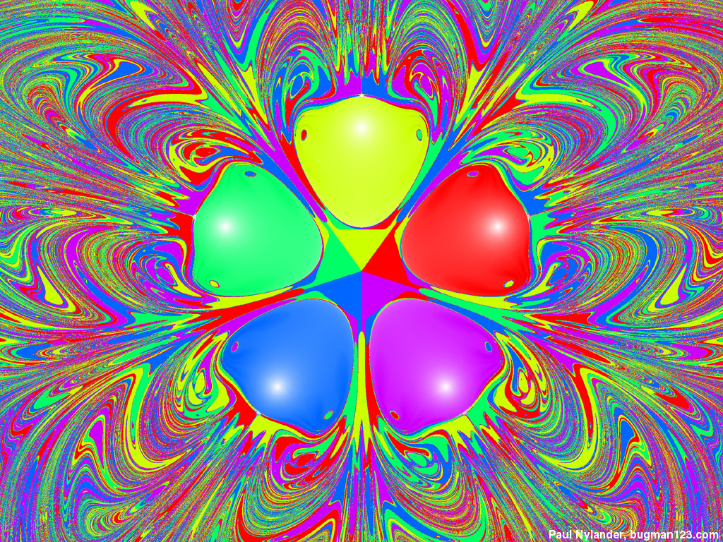The picture on the left shows another version with five magnets. See also my physics pendulums.

Here is some Mathematica code to numerically solve this using the Beeman integration scheme with the predictor-corrector modification:
(* runtime: 45 seconds, increase n for higher resolution *)
n = 40; tmax = 25; dt = 0.1; h = 0.25; g = 0.2; mu = 0.07; zlist = {Sqrt[3] + I, -Sqrt[3] + I, -2I};
image = Table[z = x + I y; v = a = a1 = 0; Do[z += v dt + (4a - a1)dt^2/6; vpredict = v + (3a - a1)dt/2; a2 = Plus @@ ((zlist - z)/(h^2 + Abs[zlist - z]^2)^1.5) - g z - mu vpredict; v += (2a2 + 5a - a1)dt/6; a1 =a; a = a2, {t, 0, tmax, dt}]; r = Abs[z - zlist]; Hue[Position[r, Min[r]][[1, 1]]/3], {y, -5.0, 5.0, 10.0/n}, {x, -5.0, 5.0, 10.0/n}];
Show[Graphics[RasterArray[image]], AspectRatio -> 1];

Links

• Magnetic Pendulum – C++ program by Ingo Berg, uses Beeman integration scheme, here is a nice big picture and here is an animation
• Mathematica code – by Urijah Kaplan
• Butterfly Effect – systems that are highly sensitive to initial conditions
• homemade magnetic pendulum – by David Williamson

3-Phase Brushless DC (BLDC) Motor

Brushless motors are popular in model airplanes. This one has a 6 pole stator and an 8 pole rotor. The technique used here is very similar to that used in Maglev trains. See also my Tesla coil magnetic field. 3-Phase Brushless DC (BLDC) Motor – POV-Ray 3.6.1, 9/31/06 Links Brushless Motor Schematics – by Gertjan Kool Finite Element Method Magnetics – free program by David Meeker

Horseshoe Magnets

These magnetic fields were made using the same technique as the solenoid picture.

new version: POV-Ray 3.6.1, 7/15/06
old version: calculated in Mathematica 4.2, rendered in TrueSpace 4.3, 3/9/03

Links

• Levitron – magnetic levitating top
• Molecular Magnetism – magnetic levitation of a frog in a Bitter solenoid
• Gravitator – magnetic levitating sphere
• Geodynamo Lab – I recently had the opportunity to tour this lab at the University of Maryland
• Electromagnetic Field in Microwave Oven – interesting discussion by Wenjun Deng (my roommate)

Magnetic Field of a Solenoid

This magnetic field was approximated by a superposition of 2D point sources using the Biot-Savart Law. You can also see the old version of this picture on Jeff Bryant’s Mathematica visualization site. Click here to download the POV-Ray code for this image. See also my magnetic field representations for a motor, Tesla coil, and horseshoe magnets.

new version: POV-Ray 3.6.1, 5/17/06; old version: calculated in Mathematica 4.2, rendered in TrueSpace 4.3, 1/19/03

(* runtime: 12 seconds *)
plist = Table[{(4 i - 26)/6, -(-1)^i}, {i, 1, 12}]; r[{xi_, yi_}] := Sqrt[(x - xi)^2 + (y - yi)^2];
DensityPlot[2Sqrt[((Plus @@ Map[#[[2]](x - #[[1]])/r[#]^2 &, plist])^2 + (Plus @@ Map[-#[[2]](y - #[[2]])/r[#]^2 &, plist])^2)] + Cos[18.8Plus @@ Map[#[[2]]/r[#] &, plist]] + 1, {x, -6, 6}, {y, -3, 3}, Mesh -> False, Frame -> False, PlotRange -> {0, 10}, PlotPoints -> {275, 138}, AspectRatio -> 1/2]

Magnet Fractals

These fractals were originally designed for predicting magnetic phase-transitions.

Here is some Mathematica code:
Mandelbrot[zc_] := Length[FixedPointList[f[#, zc] &, 0, 100, SameTest -> (Abs[#] > 2 &)]];
Magnet[] := DensityPlot[Log[Mandelbrot[xc + I yc]], {xc, -1, 3}, {yc, -2, 2}, PlotPoints -> 275, Mesh -> False, Frame -> False, ColorFunction -> (If[# != 1, Hue[#], RGBColor[0, 0, 0]] &)];

(* Magnet 1: runtime: 5 minutes *)
f[z_, zc_] := (z^2 + zc - 1.0)^2 / (2 z + zc - 2)^2;
Magnet[];

(* Magnet 2: runtime: 15 minutes *)
f[z_, zc_] := (z^3 + 3 (zc - 1) z + (zc - 1) (zc - 2))^2 / (3 z^2 + 3 (zc - 2) z + (zc - 1) (zc - 2) + 1.0)^2;
Magnet[];

POV-Ray has a built-in function for these fractals:
//Magnet 1: runtime: 0.5 second
camera{orthographic location <1.25,0,-2> look_at <1.25,0,0> angle 90}
plane{z,0 pigment{magnet 1 mandel 50 interior 1,1 color_map{[0 rgb 0][1/6 rgb <0,0,1>][1/3 rgb 1]}} finish{ambient 1}}

//Magnet 2: runtime: 0 seconds
camera{orthographic location <1,0,-2> look_at <1,0,0> angle 90}
plane{z,0 pigment{magnet 2 mandel 50 color_map{[0 rgb 0][1/6 rgb <1,0,0>][1/3 rgb 1][1 rgb 1][1 rgb 0]}} finish{ambient 1}}