

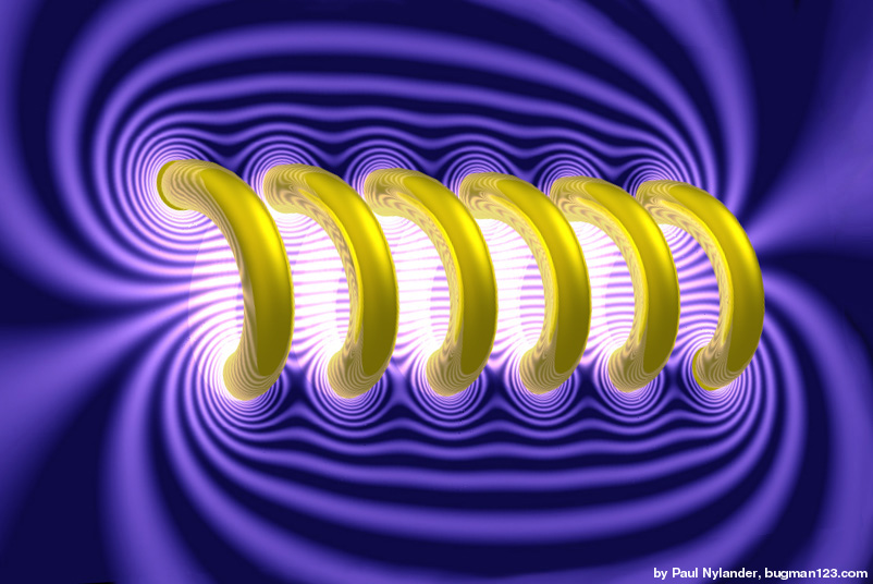
This magnetic field was approximated by a superposition of 2D point sources using the Biot-Savart Law. You can also see the old version of this picture on Jeff Bryant’s Mathematica visualization site. Click here to download the POV-Ray code for this image. See also my magnetic field representations for a motor, Tesla coil, and horseshoe magnets.

new version: POV-Ray 3.6.1, 5/17/06; old version: calculated in Mathematica 4.2, rendered in TrueSpace 4.3, 1/19/03
(* runtime: 12 seconds *)

plist = Table[{(4 i - 26)/6, -(-1)^i}, {i, 1, 12}]; r[{xi_, yi_}] := Sqrt[(x - xi)^2 + (y - yi)^2];

DensityPlot[2Sqrt[((Plus @@ Map[#[[2]](x - #[[1]])/r[#]^2 &, plist])^2 + (Plus @@ Map[-#[[2]](y - #[[2]])/r[#]^2 &, plist])^2)] + Cos[18.8Plus @@ Map[#[[2]]/r[#] &, plist]] + 1, {x, -6, 6}, {y, -3, 3}, Mesh -> False, Frame -> False, PlotRange -> {0, 10}, PlotPoints -> {275, 138}, AspectRatio -> 1/2]
 RSS feed
We would like to use your animated picture file or the still picture. Please know asap.
Thank you for your cooperation.
You have to do is simulation matlab? Already did simulation validation through Matlab for the magnetic field.
Thank you.
i like your images too much
Can you explain your Mathematica code a little bit more?