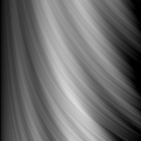
The infamous Weierstrass function is an example of a function that is continuous but completely undifferentiable.


(* runtime: 0.7 second *)

Plot3D[Sum[Sin[Pi k^a x]/(Pi k^a), {k, 1, 50}], {x, 0, 1}, {a, 2, 3}, PlotPoints -> 100];
The infamous Weierstrass function is an example of a function that is continuous but completely undifferentiable.
(* runtime: 0.7 second *)
Plot3D[Sum[Sin[Pi k^a x]/(Pi k^a), {k, 1, 50}], {x, 0, 1}, {a, 2, 3}, PlotPoints -> 100];


 Boy’s Surface (Bryant-Kusner Parametrization) : This one-sided surface was first parametrized correctly by Bernard Morin. The animation looks like it’s turning inside-out, although technically that’s impossible because it only has one side! Robert Bryant told me that the parameters (p,q) = (0,1) give this Willmore immersion of RP2 a trilateral symmetry. The parameters (p,q) = (1,0) should give bilateral symmetry. I’d like to know if it’s possible to make one with pentalateral symmetry. Click here to download some POV-Ray code for this image.
new version: POV-Ray 3.6.1, 6/20/06
old version: Mathematica 4.2, MathGL3d, POV-Ray 3.6.1, 5/24/05
(* runtime: 1 second *)

ParametricPlot3D[Module[{z = r E^(I theta), a, m}, a = z^6 + Sqrt[5]z^3 - 1; m = {Im[z(z^4 - 1)/a], Re[z(z^4 + 1)/a], Im[(2/3) (z^6 + 1)/a] + 0.5}; Append[m/(m.m), SurfaceColor[Hue[r]]]], {r, 0, 1}, {theta, -Pi, Pi}, PlotPoints -> {20, 72}, ViewPoint -> {0, 0, 1}]
POV-Ray also has an internal function for a different parametrization:
// runtime: 50 seconds

camera{location -1.5*z look_at 0} light_source{-z,1}

#declare f=function{internal(8)} isosurface{function{-f(x,y,z,1e-4,1)} pigment{rgb 1}}
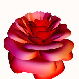  This rose is actually a plot of a single continuous math equation. Click here to see a larger animation. Click here to see a rotatable 3D version. Click here to download some POV-Ray code for this image. You can also see this on Abdessemed Ali’s web site. See also my Passion Flower.new version: POV-Ray 3.6.1, 6/21/06 This rose is actually a plot of a single continuous math equation. Click here to see a larger animation. Click here to see a rotatable 3D version. Click here to download some POV-Ray code for this image. You can also see this on Abdessemed Ali’s web site. See also my Passion Flower.new version: POV-Ray 3.6.1, 6/21/06old version: Mathematica 4.2, MathGL3d, 3/5/04
|
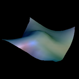
 A sphere is an elliptic surface with constant positive curvature. A pseudosphere is a hyperbolic surface with constant negative curvature. This Pseudosphere is called a Breather. Click here to download some POV-Ray code for this image. You can also see this image described as an “Imploding Flower” on Chewxy’s Math Art
new version: POV-Ray 3.6.1, 6/21/06
old version: Mathematica 4.2, MathGL3d, POV-Ray 3.6.1, 9/30/04
(* runtime: 6 seconds *)

a = 0.498888; vmax = 47.1232; w = Sqrt[1 - a^2];

Breather[u_, v_] := Module[{d = a((w Cosh[a u])^2 + (a Sin[w v])^2)}, x = -u + 2w^2 Cosh[a u]Sinh[a u]/d; y = 2w Cosh[a u](-w Cos[v]Cos[w v] - Sin[v]Sin[w v])/d; z = 2w Cosh[a u](-w Sin[v]Cos[w v] +Cos[v]Sin[w v])/d; {x, y, z, {EdgeForm[], SurfaceColor[Hue[v/vmax]]}}];

ParametricPlot3D[Breather[u, v], {u, -10, 10}, {v, 0, vmax}, PlotPoints -> {49, 79}, Compiled -> False]
 Cloth Simulation : This cloth is modelled as a net of small springs and masses. The following code still needs some improvement:
(* runtime: 2 minutes *)

Normalize[p_] := p/Sqrt[p.p]; r = 0.5; n = 13; dx = 2.0/(n - 1); dt = 0.05; g = {0, 0, -0.2};

cloth = Table[{{x, y, r}, {0, 0, 0}}, {y, -1, 1, dx}, {x, -1, 1, dx}];

Do[Show[Graphics3D[{EdgeForm[], Table[Polygon[Map[cloth[[#[[1]], #[[2]], 1]] &, {{i, j}, {i, j + 1}, {i + 1, j + 1}, {i + 1, j}}]], {i, 1, n - 1}, {j, 1,n - 1}]}, PlotRange -> {{-1, 1}, {-1, 1}, {-1, 1}}]]; Do[cloth = Table[{p1, v1} = cloth[[i, j]]; If[(i == 1 || i == n) && (j == 1 || j == n), {p1, v1},v2 = v1 + g dt; Do[i2 = i + di; j2 = j + dj; If[! (i2 == i && j2 == j) && 0 < i2 <= n && 0 < j2 <= n, L0 = dx Sqrt[(j2 - j)^2 + (i2 - i)^2]; p2 = cloth[[i2, j2, 1]]; L = Sqrt[(p2 - p1).(p2 - p1)]; v2 += (L/L0 - 1)Normalize[p2 - p1]dt], {di, -2, 2}, {dj, -2, 2}]; v2 *= 0.9; {p1 + (v1 + v2) dt/2,v2}], {i, 1, n}, {j, 1, n}], {25}], {10}];

 Loxodromes on Riemann Sphere : I made this animation in response to a special request from Donald Palermo. I am interested in finding more graphics work. Please let me know if you might have a job for me!
(* runtime: 0.7 second *)

a = 1; b = Sqrt[1 + (a t)^2];

ParametricPlot3D[{Sin[t + theta]/b, Cos[t + theta]/b, -a t/b, {EdgeForm[], SurfaceColor[Hue[t/5 - theta/Pi]]}}, {t, -10, 10}, {theta, 0, Pi}, PlotPoints -> {91, 19}]
Link: Loxodrome animation – by Frank Jones
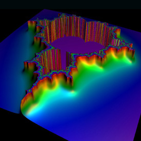 This Mandelbrot fractal was interpolated using Bill Rood’s formula for continuous escape time (cet) as described in the book “The Colours of Infinity”:
cet = n + log2ln(R) – log2ln|z|
 (* runtime: 3 seconds *)

R = 6;

image = ParametricPlot3D[Module[{z = 0.0, i = 0}, While[i < 100 && Abs[z] < R^2, z = z^2 + xc + I yc; i++]; cet = If[i != 100, i + (Log[Log[R]] - Log[Log[Abs[z]]])/Log[2], 0]; {xc, yc, 0.5Min[0.1cet, 1], {EdgeForm[], SurfaceColor[Hue[1 - 0.1cet]]}}], {xc, -2.0, 1.0}, {yc, -1.5, 1.5}, PlotPoints -> 64, Boxed -> False, Axes -> False, DisplayFunction -> Identity];

<< MathGL3d`OpenGLViewer`;

MVShow3D[image, MVNewScene -> True];

 Vibration Mode of a Spherical Membrane : This is a somewhat exaggerated example of how a spherical balloon might vibrate.
Vibration Mode of a Spherical Membrane – Mathematica 4.2, MathGL3d, 9/28/04
(* runtime: 4 seconds *)

Y := Re[SphericalHarmonicY[8, 4, theta, phi]]; r := (1 + 0.5Y);

ParametricPlot3D[{r Sin[theta] Cos[phi], r Sin[theta] Sin[phi], r Cos[theta], {EdgeForm[], SurfaceColor[Hue[Y]]}}, {theta, 0, Pi}, {phi, 0, 2Pi}, PlotPoints -> 72, Boxed -> False, Axes -> None]
31st Fundamental Mode of Vibration of a Circular Membrane. This is an example of how a circular drumhead might vibrate. Click here to see a rotatable animated version.
J3(k43r)cos(3θ) → frequency: f31 = f1k43/k10 = 6.74621 f1
(* runtime: 5 seconds *)

Clear[r]; << NumericalMath`BesselZeros`;

k = BesselJZeros[3, 4][[4]];

<< MathGL3d`OpenGLViewer`;

texture = Graphics[{RGBColor[0, 1, 1], Rectangle[{0, 0}, {10, 10}], RGBColor[0.5, 0, 1], Rectangle[{1, 1}, {9, 9}]}];

MVShow3D[ParametricPlot3D[{r Sin[theta], r Cos[theta], 0.25BesselJ[3, k r]Cos[3 theta]}, {r, 0, 1}, {theta, 0, 2Pi}, PlotPoints -> {56, 168}], MVNewScene -> True, MVTexture -> texture, MVTextureMapType -> MVMeshUVMapping, MVScaleTexture -> {14, 42}]
I hope you enjoy it!
Subscribe to the  RSS feed
 to stay informed when I publish something new here.
I would love to hear from you! Please feel free to send me an email : bugman123-at-gmail-dot-com

Recent Comments