Kleinian Double Cusp Group

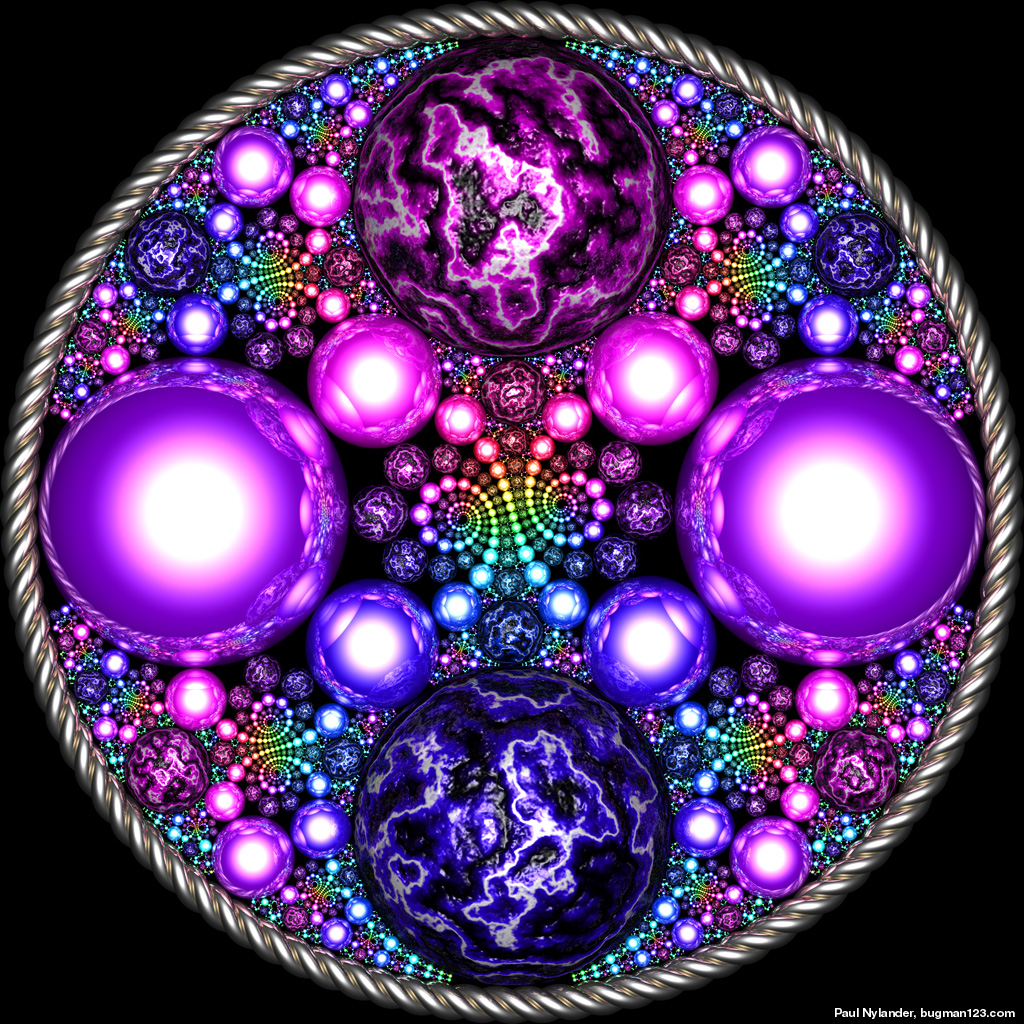
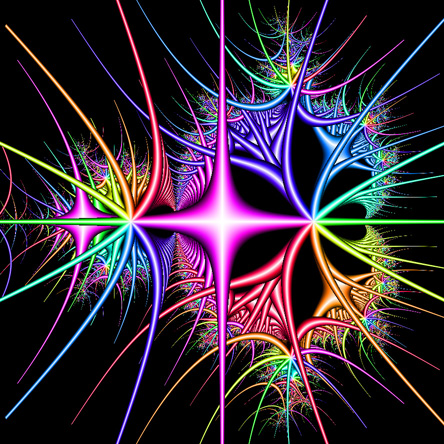
This is my attempt to create the Kleinian Double Cusp Group on page 269 of Indra’s Pearls. Thanks to Dr. William Goldman for helping me get started with this. Here is some POV-Ray code for this fractal. See also my Double Spiral. You can also see this code on Roger Bagula’s web site.

(* runtime: 0.06 second *)
ta = 1.958591030 - 0.011278560I; tb = 2; tab = (ta tb + Sqrt[ta^2tb^2 - 4(ta^2 + tb^2)])/2; z0 = (tab - 2)tb/(tb tab - 2ta + 2I tab);
b = {{tb - 2I, tb}, {tb, tb + 2I}}/2; B = Inverse[b]; a = {{tab, (tab - 2)/z0}, {(tab + 2)z0, tab}}.B; A = Inverse[a];
Fix[{{a_, b_}, {c_, d_}}] := (a - d - Sqrt[4 b c + (a - d)^2])/(2 c); ToMatrix[{z_, r_}] := (I/r){{z, r^2 - z Conjugate[z]}, {1, -Conjugate[z]}};
MotherCircle[M1_, M2_, M3_] := ToMatrix[{x0 +I y0, r}] /. Solve[Map[(Re[#] - x0)^2 + (Im[#] - y0)^2 == r^2 &, Fix /@ {M1, M2, M3}], {x0, y0, r}][[2]];
C1 = MotherCircle[b, a.b.A, a.b.A.B]; C2 = MotherCircle[b.a.a.a.a.a.a.a.a.a.a.a.a.a.a.a, a.b.a.a.a.a.a.a.a.a.a.a.a.a.a.a, a.b.A.B];
Reflect[C_, M_] := M.C.Inverse[Conjugate[M]];
orbits = Join[Reverse[NestList[Reflect[#, a] &, C1, 63]], Drop[NestList[Reflect[#, A] &, C1, 63], 1], Reverse[NestList[Reflect[#, a] &, C2, 71]], Drop[NestList[Reflect[#, A] &, C2, 56], 1]];
Show[Graphics[MapIndexed[({{a, b}, {c, d}} = #1; {Hue[#2[[1]]/15], Disk[{Re[a/c], Im[a/c]}, Re[I/c]]}) &, orbits]], PlotRange -> 35{{-1, 1}, {-1, 1}}, AspectRatio -> Automatic];

This animation shows the set morphing into a single cusp group.

Links

• Explanation – by David Wright, coauthor of Indra’s Pearls
• Kleinian Gallery – beautiful Kleinian groups by Jos Leys
• Limit Sets – interesting animations by Jeffrey Brock, see his 3D bending
• Indra’s Pearls course – Kleinian groups with David Wright
• Swirlique – program for drawing Kleinian limit sets
• Gallery – includes some nice Kleinian groups, by Curtis McMullen
• Double Spiral – POV-Ray rendering by Jeffrey Pettyjohn

Apollonian Gasket

Here are four circles inverted about each other. This is kind of similar to a Wada Basin but not exactly. Notice the small Poincaré hyperbolic tilings throughout the picture. Click here to download a Mathematica notebook for this animation. Click here to download some POV-Ray code for this fractal.

(* runtime: 0.3 second *)
chains = {N[Append[Table[{{2E^(I theta), Sqrt[3]}}, {theta, Pi/6, 9Pi/6, 2Pi/3}], {{0, 2 - Sqrt[3]}}]]};
Reflect[{z2_, r2_}, {z1_, r1_}] := Module[{a = r1^2/((z2 -z1)Conjugate[z2 - z1] - r2^2)}, {z1 + a (z2 - z1), a r2}];
Do[chains = Append[chains, Table[Map[Reflect[#, chains[[1, j, 1]]] &, Flatten[Delete[chains[[i]], j], 1]], {j, 1, 4}]], {i, 1, 6}];
Show[Graphics[Table[{GrayLevel[i/7], Map[Disk[{Re[#[[1]]], Im[#[[1]]]}, #[[2]]] &, chains[[i]], {2}]}, {i, 1, 7}], AspectRatio -> 1, PlotRange -> {{-1, 1}, {-1, 1}}]];

Links

• Circle Inversion Java applet – by Pat Hooper
• Apollonian Gasket – by Paul Bourke
• Jellyfish movie – by Curtis McMullen
• Apollonian movie – by David Dumas

Wada Basin

To make a Wada Basin, simply put some Christmas tree ornaments together.See also my Apollonian Gasket.

The following Mathematica code demonstrates how to write a very simple ray tracer:
(* runtime: 11.5 minutes *)
n = 275; r = 1; plight = {0, 0, 1}; Normalize[x_] := x/Sqrt[x.x];
spheres = {{{1, 1.0/Sqrt[3], 0}, {1, 0,0}}, {{-1, 1.0/Sqrt[3], 0}, {0, 1, 0}}, {{0, -2.0/Sqrt[3], 0}, {0, 0, 1}}, {{0, 0, -Sqrt[8.0/3]}, {1, 1, 1}}};
Intersections[p_, dir_] := Module[{a = p.dir, b}, b = r^2 + a^2 - p.p; If[b > 0, Select[Sqrt[b]{-1, 1} - a, # > 10^-10 &], {}]];
RayTrace[p_, dir_, depth_] := Module[{dlist = Map[Min[Intersections[p - #[[1]], dir]] &, spheres], d, i, p2, normal, color, lightdir, intensity}, d = Min[dlist]; If[d < Infinity, p2 = p + d dir; i = Position[dlist, d, 1, 1][[1, 1]]; normal = Normalize[p2 - spheres[[i, 1]]]; color = If[depth > 50, {0, 0, 0}, RayTrace[p2, Normalize[dir - 2(normal.dir)normal], depth + 1]]; lightdir = Normalize[plight - p2]; intensity = normal.lightdir; If[intensity > 0, shadowed = Or @@ Map[Intersections[p2 - #[[1]], lightdir] =!= {} &, spheres]; If[! shadowed,color += intensity spheres[[i, 2]]]]; color, {0, 0, 0}]];
Show[Graphics[RasterArray[Table[RGBColor @@ Map[Min[1, Max[0, #]] &, RayTrace[{0, 0, 1},Normalize[{x,y, -1}], 1]], {y, -0.5, 0.5, 1.0/n}, {x, -0.5, 0.5, 1.0/n}]], AspectRatio -> 1]];You can also easily ray trace Wada Basins using POV-Ray:
// runtime: 4 seconds
global_settings{max_trace_level 50}
camera{location z look_at 0}
light_source{z,1}
#default{finish{reflection 1 ambient 0}}
sphere{<1,sqrt(1/3),0> 1 pigment{rgb <1,0,0>}}
sphere{<-1,1/sqrt(3),0> 1 pigment{rgb <0,1,0>}}
sphere{<0,-2/sqrt(3),0> 1 pigment{rgb <0,0,1>}}
sphere{<0,0,-sqrt(8/3)> 1 pigment{rgb 1}}

Links

• Indra’s Deep Sea Life – beautiful POV-Ray images by Kevin Wampler
• Javascript Ray Tracer – simple Javascript ray tracer by John Haggerty
• another variation using a cylinder – by Paul Bourke

Flame Fractal

Flame Fractals are a popular, generalized variation of IFS fractals, invented by Scott Draves. This one is based on the ApophysisPOV-Ray code.
(* runtime: 25 seconds *)
V1[{x_, y_}] := {Sin[x], Sin[y]};
F1[p_] := Module[{p2 = {{0.81, -0.33}, {0.08, 0.89}}.p + {0.24, -0.07}}, 0.88p2 + 0.12V1[p2]];
F2[p_] := Module[{p2 = {{0.3, 0.52}, {-0.56, 0.37}}.p + {-0.09, -0.42}}, 0.88p2 + 0.12V1[p2]];
F3[p_] := V1[{{-0.43, 0.38}, {-0.2, -0.44}}.p + {1.74, 1.21}];
F4[p_] := V1[{{-0.49, -0.27}, {0.28, -0.53}}.p + {0.51, 0.62}];
w1 = 0.65; w2 = 0.29; w3 = 0.03; w4 = 0.03;
n = 275; image = Table[{0, 0, 0}, {n}, {n}]; p = {0, 0};
Do[x = Random[]; k = Which[x < w1, 1, x < w1 + w2, 2, x < w1 + w2 + w3, 3, True, 4]; p = {F1, F2, F3, F4}[[k]][p]; {j,i} = Round[n{p[[1]] + 1.1, p[[2]] + 1.8}/3]; image[[i, j]] += List @@ ToColor[Hue[k/4.0], RGBColor], {100000}];
Show[Graphics[RasterArray[Map[RGBColor @@ Map[(1 - Exp[-0.2#]) &, #] &, image, {2}]], AspectRatio -> 1]];

Links

• Cory Ench – some impressive flame fractals
• Apophysis – free Flame Fractal software
• Flame Fractal Java applet sample parameters. See also my inefficient

Golden Ratio Spiral Orbit Trap

Here is an Orbit Trap in the shape of the Golden Ratio Spiral.

(* runtime: 1 minute *)
phi = 0.5(1 + Sqrt[5]);
f[z_] := Module[{r = Log[Abs[z]]/(4Log[phi]) - Arg[z]/(2Pi)}, 18Abs[r - Round[r]]];
OrbitTrap[zc_] := Module[{z = 0, i =0}, While[i < 100 && Abs[z] < 100 && (i < 2 || f[z] > 1), z = z^2 + zc; i++]; Hue[Arg[z]/(2Pi), Min[1, 2 f[z]], Max[0, Min[1, 2(1 - f[z])]]]];
Show[Graphics[RasterArray[Table[OrbitTrap[xc + I yc], {yc, -1.5, 1.5, 3.0/275}, {xc, -2, 1, 3.0/275}]], AspectRatio -> 1]];

Circular Orbit Trap

This animation shows a Circular Orbit Trap transforming into a biomorph.
(* runtime: 12 seconds *)
OrbitTrap[zc_] := Module[{z = 0, i = 0, x}, While[i < 10 && Abs[z] < 2 && (i < 2 || Abs[z] > 0.3), z = z^2 + zc; i++]; x = Abs[z]^2/0.3^2; Hue[Arg[z]/(2Pi), Min[1, 2 x], Max[0, Min[1, 2(1 - x)]]]];
Show[Graphics[RasterArray[Table[OrbitTrap[xc + I yc], {yc, -1.5, 1.5, 3/274}, {xc, -2.0, 1.0, 3/274}]], AspectRatio -> 1]];

Mandelbrot Set Pickover Stalks

Pickover stalks are cross-shaped orbit traps invented by Clifford Pickover. See also my 3D Pickover stalks fractals. Here is some Mathematica code:
(* runtime: 33 seconds *)
f[z_] := Min[Abs[{Re[z], Im[z]}]]/0.03;
OrbitTrap[zc_] := Module[{z = 0, i = 0}, While[i < 100 && Abs[z] < 100 && (i < 2 || f[z] > 1), z = z^2 + zc; i++]; Hue[Arg[z]/(2Pi), Min[1, 2 f[z]], Max[0, Min[1, 2(1 - f[z])]]]];
Show[Graphics[RasterArray[Table[OrbitTrap[xc + I yc], {yc, -1.5, 1.5, 3/274}, {xc, -2.0, 1.0, 3/274}]], AspectRatio -> 1]]

Links

• Biomorphs – biological-looking Pickover stalks, by Paul Bourke
• Dragon on a Pedestal – by Damien Jones

Cubic Julia Set Fractal

z_n+1 = z_n³+z_c, z_c = -0.5-0.05i
This was one of my older favorites.

original version: Java, 6/9/01;
animated version: Mathematica 4.2, 2/18/05

(* runtime: 10 seconds *)
Julia = Compile[{{z, _Complex}}, Length[FixedPointList[#^3 + zc &, z, 100, SameTest -> (Abs[#] > 2 &)]]];
zc = -0.5 - 0.05 I;
DensityPlot[Julia[x + I y], {x, -1.15, 1.15}, {y, -1.15, 1.15}, PlotPoints -> 275, Mesh -> False, Frame -> False, ColorFunction -> (RGBColor[Min[2#^2, 1], Max[2# - 1, 0], Min[2#, 1]] &)];

This is how you can make this fractal in POV-Ray:
// runtime: 0.5 second
camera{orthographic location <0,0,-1.15> look_at 0 angle 90}
plane{z,0 pigment{julia <-0.5,-0.05>,30 exponent 3 color_map{[0 rgb 0][1/3 rgb <0,0,1>][2/3 rgb <1,0,1>][1 rgb 1]}} finish{ambient 1}}

Mandelbrot Set Zoom

z_n+1 = z_n²+z_c
This animation zooms in on the Mandelbrot set by a factor of 10¹⁵. At this high resolution, double precision numbers are inadequate. Therefore, this animation was created using “double-double” precision numbers, adapted from Keith Brigg’s double-doubles. See also my Java program and C program.

Mandelbrot Set Zoom – original version: Java, 5/24/01; animated version: C++, 2/16/05 Here is some Mathematica code for this fractal:
(* runtime: 1 minute *)
Mandelbrot[zc_] := Module[{z = 0, i = 0}, While[i < 100 && Abs[z] < 2, z = z^2 + zc; i++]; i];
DensityPlot[Mandelbrot[xc + I yc], {xc, -2, 1}, {yc, -1.5, 1.5}, PlotPoints -> 275, Mesh -> False, Frame -> False, ColorFunction -> (If[# != 1, Hue[#], Hue[0, 0, 0]] &)];

Here is a faster version:
(* runtime: 7 seconds *)
Mandelbrot = Compile[{{zc, _Complex}}, Length[FixedPointList[#^2 + zc &, zc, 100, SameTest -> (Abs[#] > 2 &)]]];
DensityPlot[Mandelbrot[xc + I yc], {xc, -2, 1}, {yc, -1.5, 1.5}, PlotPoints -> 275, Mesh -> False, Frame -> False, ColorFunction -> (If[# != 1, Hue[#], Hue[0, 0, 0]] &)];

POV-Ray has a built-in function for this fractal:
// runtime: 0.5 second
camera{orthographic location <-0.5,0,-1.5> look_at <-0.5,0,0> angle 90}
plane{z,0 pigment{mandel 100 color_map{[0 rgb 0][1/6 rgb <1,0,1>][1/3 rgb 1][1 rgb 1][1 rgb 0]}} finish{ambient 1}}

Links

• Deep-zooming – Fractint can zoom in by magnification factors of up to 10¹⁶⁰⁰
• 1/50 of a Light Year – zooming animation by Damien Jones (10¹⁵)

Frequency Filtered Random Noise

Frequency Filtered Random Noise : another variation of frequency filtered random noise.
(* runtime: 20 seconds *)
n = 275; SeedRandom[1]; fourier = Fourier[Table[Random[], {n}, {n}]];
filter = Table[fourier[[i, j]]/((j/n - 0.5)^2 + (i/n - 0.5)^2), {i, 1, n}, {j, 1, n}];
ListDensityPlot[Map[Abs, InverseFourier[filter], {2}], Mesh -> False, Frame -> False, ColorFunction -> (Hue[# + 0.5] &)];